Positional quality assessment based
on linear elements
Evaluación de calidad posicional basada en elementos lineales
Antonio Tomás Mozas-Calvache1
Recibido 14 de diciembre de 2020; aceptado 21 de febrero de 2021
Abstract
This study describes the current state of the art related to the assessment of the positional accuracy of spatial databases based on lines. The use of this type of element of spatial databases has increased in recent years because of the current possibilities of acquisition and sharing data of routes, roads, etc. Nowadays, users are also contributors and this supposes that the spatial quality of data acquired and shared by non-experts must be assessed as is the case with data produced by institutions and enterprises. In this context, several methods based on lines have been developed up to this time for several purposes. This study reviews these methods, analyzing their characteristics, measures, etc. In addition, more than 30 applications of these methods are also summarized. These applications include control of generalized and digitized lines, control of spatial databases, analysis of the displacement of lines between dates, etc.
Key words: lines, positional accuracy, quality, spatial databases, assessment.
Resumen
Este estudio describe el estado actual del arte relacionado con la evaluación de la exactitud posicional basada en líneas. El uso de este tipo de elementos de las bases de datos espaciales se ha incrementado en los últimos años debido a las posibilidades actuales de adquisición e intercambio de datos espaciales de rutas, carreteras, etc. Hoy en día, los usuarios también son contribuyentes y esto supone que la calidad espacial de los datos, adquiridos y compartidos por personas no expertas, deben evaluarse como se hace con los datos espaciales producidos por instituciones y empresas. En este contexto, se han desarrollado varios métodos basados en líneas hasta este momento para varios propósitos. Este estudio repasa estos métodos, analizando sus características, métricas, etc. Además, también se resumen más de 30 aplicaciones de estos métodos desarrollados hasta el momento. Las aplicaciones incluyen el control de líneas generalizadas y digitalizadas, el control de bases de datos espaciales, el análisis del desplazamiento de líneas entre fechas, etc.
Palabras clave: líneas, exactitud posicional, calidad, bases de datos espaciales, evaluación.
1. Introduction
This article summarizes the main methods and applications developed, until this moment, for assessing and/or controlling the positional accuracy of spatial databases based on lines. Positional accuracy is one of the main components of quality related to spatial databases (Mozas-Calvache & Ariza-López, 2011). Other components include attribute accuracy, temporal accuracy, logical consistency and completeness (ISO, 2013). This study is focused on positional accuracy and more specifically on its assessment based on linear elements. A line can be defined by a set of ordered vertexes that are connected by segments. The use of lines supposes an important alternative to the traditional controls based on points both independently or in a complementary way. There are several methods and standards published by several authors and institutions during the last decades which use a sample of well-distributed points (USBB, 1947; ASCE, 1983; ASPRS, 1990; FGDC, 1998) to determine the positional accuracy of cartographic products. In general, the coordinates of these points are compared to those obtained from more accurate sources using several metrics (e.g. Root Mean Squared Error, RMSE). However, there are several aspects to be considered related to the positional accuracy of spatial databases. Firstly, there are more types of elements in a spatial database such as lines or polygons. In fact, lines suppose the large group in a spatial database (Cuenin, 1972) and they usually have a good spatial distribution over any area (Mozas-Calvache & Ariza-López, 2014). Secondly, the analysis of these elements can improve the results of the assessment because of their own spatial characteristics. Lines contain a great deal of geometrical information defined by a large quantity of vertexes (Mozas & Ariza, 2011). Despite the fact that lines are commonly well-distributed and well-defined on a map, producers and institutions have traditionally used points to check the positional accuracy. Maybe this selection was caused by the best definition of these elements, both in the database and in reality, and the ease of determination of the coordinates using classical surveying, including static observations performed using Global Navigation Satellite System (GNSS). Nowadays the acquisition of lines from a more accurate source has achieved a great improvement thanks to the evolution of the acquisition devices and to the development of kinematic measuring techniques. Lines are acquired much more comfortably and quickly Ruiz-Lendínez et al. (2009). Definitely, the use of linear elements can be considered for assessing the positional accuracy of spatial databases. This premise has been analysed during recent years by several authors.
The quality requirement of spatial databases has undergone a great development during the last few decades. This tendency has been based mainly on the growing concern of producers and users for the quality of products and services and the increase of the availability of the geographic information (GI) on the Internet, which implies a greater demand of data quality on the part of producers and users. An example of this increase of availability on the Internet is the development and establishment of Spatial Data Infrastructures, which allow users to access GI easily. As a consequence, the demand of GI has expanded to those user segments who were not used to these type of products in the past. In addition the global distribution of mobile devices, which has greatly eased positioning measurement, and consequently the development of location-based services, has obviously contributed to this expansion. Nowadays, this evolution supposes a change of paradigm because GI is no longer solely generated by traditional producers. Thus, users are producing, sharing and consuming geospatial data continuously. Goodchild (2007) suggested the term Volunteered Geographical Information (VGI) to include those data produced by citizens in this context. As an example, VGI includes routes and tracks surveyed and shared by users on applications such as OpenStreetMap, Wikiloc, etc. Consequently, we must consider that a large amount of VGI data are composed of lines. Obviously, the positional quality of this data must also be controlled because users require a level of quality similar to that demanded for data produced by institutions. This large amount of GI continually added and updated requires new mechanisms to control their quality feasibly and rapidly. In this context, the methods based on lines have a wide field of application. Antoniou & Skopeliti (2015) gave a more detailed description of measures and indicators of VGI quality.
During recent years the necessity of using lines to assess spatial databases has definitely intensified, both generally (a complete database) and particularly (several sets of elements represented by lines). Some examples of these particular assessments are the control of digitized lines, simplified lines, matching between vector datasets, the determination of displacements between dates, etc. Essentially, any application where two sets of lines must be compared spatially. This necessity has allowed the development of several methods for controlling the positional accuracy of a sample of these elements. In this study most of these methods are described in the methodology section and their main applications are described in the results section. Previously to their description it is necessary to understand how they have been developed based on the concept of uncertainty of lines based on their spatial characteristics. In this context several uncertainty models have been described until now for segments, and consequently for lines (Figure 1). The first model used to describe the uncertainty of digitized lines was the concept of the epsilon band. This was initially proposed by Perkal (1956) and subsequently adapted by several authors (Chrisman, 1982; Blakemore, 1984; Goodchild, 1987; Hunter & Goodchild, 1995; Leung & Yan, 1998; Kronenefeld, 2011). The concept of the epsilon band supposes the true position of a line included inside a certain displacement (epsilon) from the position of the digitized line. Geometrically, it is defined by two lines parallel to the most probable position and tangential to the circular error at the extreme vertexes of each segment (Figure 1a). This supposes a normal-circular distribution of error at the extremes of the segment. From the first definition the epsilon band model has been improved to include variable width in the intermediate points of the segment (Caspary & Scheuring, 1993) (Figure 1b), nearer to a theoretical model of probability distribution (Winter, 2000) (Figure 1c). Caspary & Scheuring (1993) proposed a simplified error band with the minimum positional error shown in the midpoint of the segment (Gil de la Vega et al., 2016) (Figure 1b). In addition to these models, Shi & Liu (2000) proposed the G-band considering that infinite points compose the line. They assumed that the errors at the extreme points follow normal distributions. In addition, the errors in these points can be correlated to each other and the intermediate points of the segment are stochastically continuous to each other (Figure 1d). Other models represent uncertainty with probability distribution functions (Heuvelink et al., 2007; Wu & Liu, 2008). Gil de la Vega et al. (2016) carried out a more detailed description of these models and their adaptation to the 3D case.
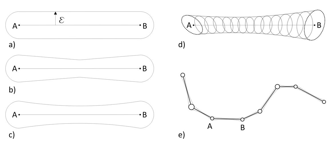
Figure 1. Uncertainty models of segements and lines: a) epsilon band; b) and c) error band; d) G-band; e) error band of a line.
In addition to these uncertainty models, several studies were undertaken to analyse positional effects caused by the simplification process based on the geometry of lines. These studies described interesting metrics for performing a positional control. McMaster (1986) described several metrics such as the percentage change of length, the ratio of change in the number of coordinates, the difference in average number of coordinates per inch and the ratio of change in the standard deviation of the number of coordinates per inch, the percentage change of angularity and the ratio of change in the number of curvilinear segments. McMaster (1986) included two comparative metrics in order to analyse the displacement between both lines (original and simplified). These metrics can be considered basic to the development of positional control methods. The first is the vector displacement, calculated by the sum of the length of all vectors divided by the length of the original line. The second is the areal displacement, which is determined by the sum of the areas of the polygons formed between the original and the simplified lines divided by the length of the original line. Jasinski (1990) extended these metrics to include the error variance, the average segment length and the average angularity. Veregin (2000) described the uniform distance distortion based on the distortion polygons (areas) enclosed by both lines. Ramirez & Ali (2003) described other interesting metrics such as the bias factor, the distortion factor, the fuzziness factor and the generalization factor.
Another aspect to consider when assessing the positional accuracy of any spatial database based on lines is related to the sample of the elements to be used. The selection of a sample of lines must consider the characteristic of the population in order to obtain similar results using the selected sample. Ruiz-Lendínez et al. (2009) described three phases: establish a population of interest, estimate the size of the population and determine the size of the sample. In this sense, Ariza-López et al. (2011) studied the size of a sample of lines based on a simulation process using roads. In this process they used several methods to assess positional accuracy based on lines.
Traditionally, the assessment of the positional accuracy of the spatial databases has been carried out using points both in 2D and in 3D. The application of the different metrics to heights supposed in the majority of cases a simple addition of the Z coordinate to the metrics applied to the horizontal component. However, the study of the vertical accuracy (heights) was usually carried out independently with respect to the horizontal accuracy (USBB, 1947; ASCE, 1983; ASPRS, 1990; FGDC, 1998). Among others, this was caused by the different spatial behaviour and representation of heights (e.g. contour lines, Digital Elevation Models, etc.). In the case of linear elements, the first metrics were developed to assess the positional accuracy of lines obtained from digitizing or generalization. So initially, the control of the vertical accuracy was not implemented. However, with the development of 3D spatial databases and the availability of control lines obtained directly from GNSS kinematic surveys (defined by 3D vertexes), Mozas-Calvache & Ariza-López (2015) included the vertical component in this type of assessment by adapting some metrics based on lines. In most cases the inclusion of the vertical component supposed the development of a new procedure for adapting previous metrics developed for 2D.
This study reviews the methods and applications based on lines developed during recent decades to assess the positional accuracy of a set of lines or a complete spatial database. The use of these types of elements is widely justified considering the current development of technology and the large amount of spatial data available on the Internet.
2. Methods
The firsts studies published on the assessment of the positional accuracy of lines were developed to analyse digitized and generalized lines. After that, several methods were developed to assess the positional quality of spatial databases. Previous studies have included some classifications of these methods, such as Atkinson-Gordo & Ariza-López (2002), Santos et al. (2015) and Gil de la Vega et al. (2016). In this study, we are going to update and review them following the classification shown by Mozas-Calvache & Ariza-López (2015) and Gil de la Vega et al. (2016), which differentiated between methods based on line-to-line distance measures (EBM, ADM, HDM, VIM, VIM-V) (Figure 2) and methods based on buffered lines (SBOM, DBOM) (Figure 3).
All methods are based on a set of lines to be assessed (XL) and the homologous set of lines obtained from a more accurate source used as reference (QL).
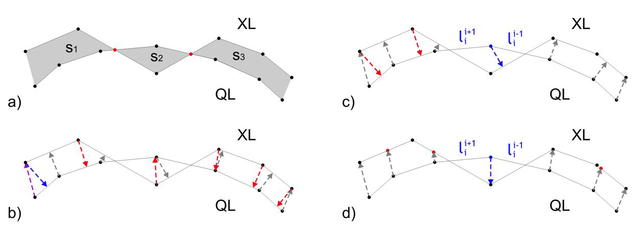
Figure 2. Methods based on line-to-line distance measures: a) EBM; b) ADM and HDM; c) VIM; d) VIM-V.
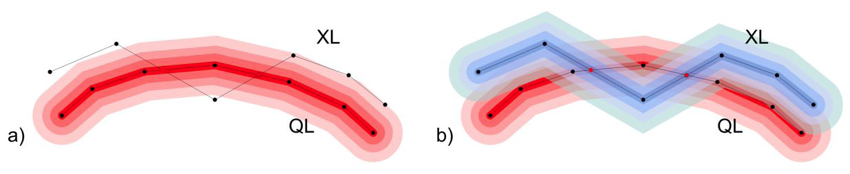
Figure 3. Methods based on buffered lines: a) SBOM; b) DBOM.
2.1. Methods based on line-to-line distance measures
2.1.1. Epsilon Band Method (EBM)
The Epsilon Band Method was based directly on the metrics developed by McMaster (1986). It consists of the determination of the enclosed area between both lines XL and QL (S=S1+S2+S3 in Figure 2a) and division by the length of the line to be controlled (XL). The calculation of the enclosed area is based on the sum of all sub-areas determined by two consecutive crosses between both lines. This metric initially was applied to the study of generalized lines but Skidmore & Turner (1992) adapted it to control the displacement between two lines. Several authors have also used this method to obtain a mean displacement between both lines, such as Veregin (2000) and Mozas & Ariza (2010). In addition, Mozas-Calvache & Ariza-López (2015) expanded the use of this method from 2D to 3D. In this case, the calculation of the area was based on a 3D triangulation between both lines (XL and QL).
2.1.2. Average Distance Method (ADM)
This method was described by McMaster (1986) to study the positional quality of the generalization process and was applied by Mozas-Calvache & Ariza-López (2010) to control the positional accuracy of a set of roads. It is based on the calculation of the Euclidean distance between the vertexes of the XL line to the nearest point of the QL line and vice versa (see red and grey arrows in Figure 2b). The mean displacement between both lines is obtained considering the average distance determined. So the Euclidean distance is calculated from each vertex of a line to the nearest point of the other line. This nearest point on the other line can be defined by a vertex or by an intermediate point of a segment. In this case, the distance is perpendicular to the segment in that point (Figure 2b). Mozas-Calvache & Ariza-López (2015) expanded this method to 3D, including height values in all calculations.
Lawford (2010) developed an adaptation of this method. In this case, the line is divided by a defined interval of length. The points determined by these intervals are used to obtain the values of the distances (offsets) with respect to the other line. Therefore they used a set of points distributed along the XL line, with a certain separation between them to obtain the distances to the other line (QL line). This method allows us to obtain a probability distribution of displacements. The result included the value of the 90th absolute percentile of offset distances.
2.1.3. Hausdorff Distance Method (HDM)
The Hausdorff distance gives a measure of proximity between two lines (XL and QL). Hangouët (1995) described some properties of this metric such as asymmetry, orthogonality, sensitivity, tricks and tangency. Abbas et al. (1995) used this metric to assess linear elements. The Hausdorff distance indicates the maximal distance between any vertex of one line to the other and vice versa. The value of the Hausdorff distance is the greatest of both maximum values of distances. As in the case of previous methods, Mozas-Calvache & Ariza-López (2015) expanded the use of this metric to 3D lines. This method has been applied in matching procedures of linear elements Xavier et al. (2016).
2.1.4. Vertex Influence Method (VIM)
Mozas & Ariza (2011) developed the vertex influence method. It consist of the determination of a mean value of displacement between both lines. First, the Euclidean distances between the vertexes of the QL line with respect to the XL line are calculated. Each distance is weighted by the length of the two segments adjacent to the implicated vertex (Figure 2c). So the final value of displacement is obtained from a weighted mean: summing up all values obtained in each vertex and dividing this sum by the double of the length of the QL line. Using this method the displacements (distances) from vertexes with longer adjacent segments are emphasized with respect to those that have less length.
An interesting metric added by Mozas & Ariza (2011) was the study of the components of the displacement vectors that define the distances. So they analysed each component (X and Y) of the displacement vectors independently. The goal was to detect positive and negative increments in these components and consequently to detect the presence of biases in the displacement between both lines. Similar to the case of the distances, the components values were also weighted by the length of the segments adjacent to the implicated vertex.
Mozas-Calvache & Ariza-López (2015) expanded both metrics to the 3D case. The result of this adaptation allows the determination of a mean 3D displacement between both lines.
2.1.5. Vertex Influence Method by Vertexes (VIM-V)
This method was derived from the previous one. In this case, Mozas-Calvache & Ariza-López (2018) suggested the application of the VIM method to calculating the distances and components between the vertexes of the QL line and their homologous vertexes of the XL line. The main goal was the determination of biases because lines can hide these type of displacements when the direction is coincident to the direction of the line. The method includes a previous procedure for determining homologous points in the XL line to those vertexes of the QL line. It consists of the adaptation of the turning function (Arkin et al., 1991) to identifying homologous vertexes using three parameters based on distance and angles. After that, an interpolation in the XL is carried out to obtain points in this line that match those vertexes of QL which are not homologous. Finally, the VIM method is adapted using the calculations between homologous vertexes (from QL to XL) instead of between the vertexes of QL to the XL line (Figure 2d).
2.2. Methods based on buffered lines
2.2.1. Single Buffer Overlay Method (SBOM)
Goodchild & Hunter (1997) described the Single Buffer Overlay Method. The idea is to apply the concept of the uncertainty band directly to the assessment of positional accuracy. It consists of the generation of a buffer with a defined width around the QL line and the calculation of the percentage of the length of the XL displayed inside this buffer. A probability distribution is obtained with the percentage of inclusion obtained after increasing the buffer’s width. Considering this method, Mozas-Calvache & Ariza-López (2010) added a secondary measure based on the percentage of vertexes included inside the buffers after the increase of the width. Analogically to the case of the length, they obtained a probability distribution of inclusion of vertexes depending on the width. This method has been widely applied to controlling spatial databases, to assessing VGI data, in matching procedures, etc.
2.2.2. Double Buffer Overlay Method (DBOM)
Tveite & Langaas (1999) described the Double Buffer Overlay Method. It consists of the generation of a buffer (with a defined width) around each line (XL and QL) and the analysis of the possible situations derived from their spatial behaviours and intersections. After that, the buffers’ width is increased in a similar way to the previous method in order to obtain a distribution of results. So they examined 4 types of areas generated by the buffers: outside both buffers, inside the QL buffer and outside the XL buffer, inside the XL buffer and outside the QL buffer and inside both buffers. Using these measures, they proposed several metrics for each buffer width (e. g. average displacement, oscillation, etc.). Finally, a distribution function is obtained for these measures based on the buffers’ width.
3. Applications and results
During the last decades some studies have used positional control methods based on lines to assess sets of linear elements or spatial databases. In this study we summarize the main applications carried out and their results. To be coherent with the evolution of the methods, in this summary the applications are described ordered by their date of appearance.
- Abbas et al. (1995) applied the HDM to a set of routes (266 elements) and railways (101 elements) selected from a zone of about 6 by 8 km. The length of these elements was between 100 m and 1000 m. The XL set of lines was obtained from the IGN-DBcarto (France) at scale 1:30 000 and the QL set of lines was obtained from the IGN-BDTopo at scale 1:17 000. The results show a RMSE value of about 10,67 m.
- Goodchild & Hunter (1997) tested the SBOM method using a set of 179 km of coastline from the Digital Chart of the World at 1:1 000 000 (XL lines). As reference (QL lines) they used a set of lines digitized from local topographic maps at 1:25 000. The results show a distribution function that related buffer width to the percentage of inclusion. For example, they obtained that a 95% inclusion rate was obtained using a buffer width of about 400 m.
- Kagawa et al. (1999) used the SBOM and the HDM with a set of roads (706,8 m) obtained from aerial surveys at scale 1: 2500 (XL lines) and a set of lines digitized from another source at scale 1:500 (QL lines). The results of SBOM show about 1,99 m with 95% of inclusion. In addition, the results of HDM show a value of 4,3 m.
- Tveite & Langaas (1999) tested the DBOM method using four datasets of roads, coastline data and railways from the Digital Chart of the World at scale 1:1 000 000 (XL lines) and as reference, the Norwegian N250 at scale 1:250 000 (QL lines). They obtained several distribution functions for each case and each measure described in DBOM (accuracy, average displacement, oscillation and completeness). For example, the accuracy of road data was about 1600 m (buffer’s width at 70%).
- Johnston et al. (2000) applied the SBOM method to assessing the Fort Hood ITAM database. More specifically, they assessed roads and hydrology (XL lines) using lines extracted from imagery as reference source (QL). As an example, the results showed values of 94,70% of inclusion inside the buffer of 100 m in case of the roads.
- Tsoulos & Skopeliti (2000) used the HDM method to assess the digitization performed by eighteen operators using a coastline derived from a 1:1 000 000 scale map. They segmented the coastline into five segments. The results show values of maximum distance from 18,53 m to 37,73 m in these cases.
- Van Niel & McVicar (2002) applied the DBOM to assessing the positional accuracy of roads of the Digital Topographic Data Base of Australia at scale 1:50 000 (XL lines). The reference dataset (QL lines) was composed of a set of lines obtained from the centreline of over 466 km of road obtained using DGPS. The results showed that 95% of the roads were within 50 m.
- Kounadi (2009) assessed the positional quality of the OSM road network (XL lines) using as reference the Hellenic Military Geographical Service (HMGS) dataset (QL lines). The zone located in the Athens area was divided into 25 tiles of about 1 km2. The selected method was SBOM using a buffer sizes of 7,5 m, 5 m and 4 m depending on the type of road. As an example, in the Athens tile, composed of more than 209 km of roads, the average overlap was about 89,54%.
- Haklay (2010) used the SBOM method to evaluate the positional accuracy of OSM roads in England (XL lines). He used the Ordnance Survey Meridian dataset that provides coverage of Great Britain at scales 1:1 250, 1:2 500 and 1:10 000 (QL lines). The results using 1 m of buffer width showed values of inclusion from 59,81% to 88,80% with an average value of nearly 80%.
- Lawford (2010) applied an adaptation of the ADM using intervals of 100 m to determine the distances between both lines. He assessed several datasets from Geoscience Australia (at scales 1:250 000, 1:1 000 000, 1:2 500 000, 1:5 000 000, and 1:10 000 000) (XL lines) using as reference a dataset from the Victorian Department of Sustainability and Environment at scale 1:25 000 (QL lines). The results showed the 90th percentile absolute of the offset distances. For example, a value of 142,41 m was obtained for roads of the 1:250 000 dataset.
- Mozas-Calvache & Ariza-López (2010) described the results of applying several methods (EBM, ADM, HDM, SBOM and DBOM) to two datasets (Mapa Topográfico de Andalucía-MTA at scale 1: 10 000 and Mapa Topográfico Nacional-MTN at scale 1:25 000) (XL lines). The selected sample of lines was composed of more than 3300 km of roads. The reference dataset was obtained using a GNSS kinematic survey (QL lines). The results showed mean displacement of about 4,2 and 4,4 for MTA and 3,1 and 3,4 m for MTN using EBM and ADM respectively. The HDM showed maximum values of 11 m in both databases. In addition, the application of the SBOM showed that 95% inclusion was reached using 10 m in both cases. The results of DBOM showed average displacements of about 6,5 m and 4,7 m for MTA and MTN respectively.
- Zhang et al. (2010) used the SBOM to assess a set of GNSS traces of roads obtained from OSM. These roads were represented by the centreline (XL lines), determined using a method for integrating traces developed by these authors. As reference, they used the roads obtained from the TeleAtlas dataset. The results showed a percentage of inclusion of about 74% at 7 m of buffer width.
- Girres, J. F., & Touya, G. (2010) used the EBM and HDM to assess the positional accuracy of 93 km of roads obtained from OSM in France (XL lines). As reference dataset they used the homologous linear objects obtained from IGN-BDTOPO. The results showed mean values of 2,19m (EDM) and 13,57 m (HDM).
- Mozas-Calvache & Ariza-López (2011) tested the VIM using a sample of more than 180 km of roads from a database at scale 1: 100 000 (DEA100) (XL lines). As reference they used another database at scale: 1:10 000 (MTA) (QL). The results of applying VIM showed an average displacement of about 5,2 m. The analysis of components X and Y show distribution with mean values of about -1 m in X and 0,07 m in Y. The authors also applied EBM, ADM, HDM, SBOM and DBOM, obtaining interesting results. In addition, they also applied some of these methods to a set of synthetic lines affected by simulated displacements in order to compare the results of the average displacement obtained.
- Ariza-López et al. (2011) applied EBM, HDM, SBOM and DBOM in a simulation process using sample sizes of road axes from 10 km to 200 km. The goal was to determinate the influence of sample size on these methods. They used a set of 1210 km of lines of the MTA at scale 1:10 000 (XL lines) which was controlled by a dataset obtained using a GNSS kinematic survey (QL lines). The results demonstrated the viability of the simulation process developed in the study and suggested sample sizes depending on the method applied.
- Ariza-López & Mozas-Calvache (2012) applied the EBM, HDM, SBOM and DBOM to a set of twelve synthetic lines affected by certain simulated perturbations (bias, random errors and outliers). The results allowed them to determine the efficiency of each method in detecting the perturbations applied to the lines.
- Mozas-Calvache et al. (2012) applied EBM, HDM and SBOM to 4 km of a road extracted from a Quickbird scene (XL lines). The reference set of lines was obtained from a more accurate GNSS kinematic survey (QL lines). The results showed values of 2,7 of maximum displacement, 0,92 m of mean displacement and buffer widths of 0,8 m, 1,8 m and 2,2 m, considering 50%, 90% and 95% of inclusion respectively.
- Mozas-Calvache et al. (2013a) used an adaptation of the SBOM method to control four sets of contour lines at different intervals derived from a DEM at 10 m (XL lines). In addition, another dataset of contour lines was also used (obtained from the MTN at 1:25 000) (XL lines). As reference, they used a set of control points obtained from the DEM. The adaptation of the SBOM proposed by these authors supposed the generation of a 3D buffer around the maximum slope line between two consecutive contour lines and the determination of the percentage of inclusion of the control points inside this buffer. As occurred with the SBOM, the width of the buffer was increased to obtain a distribution of inclusions of the points. The results showed best behaviour in contour lines datasets with lower interval and higher slopes. In the case of the MTN, 90% of inclusion was reached using 35 m, which was coherent to that obtained using NSSDA standard based on points (39 m of RMSE at 95%).
- Ruiz-Lendínez et al. (2013) applied the SBOM and the DBOM to assessing the positional accuracy of the perimeter of urban polygons of the BCN dataset at scale 1:25 000 (XL lines) using as reference those matched polygons from the MTA at scale 1:10 000 (QL lines). The results showed uncertainties (95%) from 9,2 to 16,1 m using SBOM and average displacements from 4,6 to 6,3 m depending on the zone.
- Mozas-Calvache et al. (2013b) applied the VIM to quantifying planimetric changes of river channels between two dates. The line datasets were obtained from two orthoimages. Both banks of the river were digitized and an axis for each date was obtained segmented into several lines. Finally, both axes were compared using VIM and the results showed values lower than 50 m in the majority of cases.
- Arsanjani et al. (2013) applied the SBOM to assessing the positional accuracy of more than 2624 km of road networks obtained from OSM (XL lines). Lines obtained from the Federal Agency for Cartography and Geodesy (BKG) of Germany composed the reference dataset (QL lines). To apply this method they used buffer widths of 3, 5, 10 and 15 m.
- Mozas-Calvache & Ariza-López (2014) used the VIM to determine the systematic displacement of a sample of roads obtained from a database at scale 1: 10 000 (MTA). The sample of lines, composed of more than 180 km, was affected by simulated disturbances (translations, rotations, scaling, etc.) (XL lines). The reference was composed of the original dataset of lines (QL). Definitely, the authors determined 17 cases to be controlled using VIM. They obtained the results of the displacement vectors using VIM and based on these results they determined the presence of bias (using Student’s t-test) in the cases related to translations and rotations.
- Eshghi & Alesheikh (2015) used the SBOM to assess the positional accuracy of VGI lines of roads in Tehran (Iran). The reference dataset was obtained from organizations. The results showed the length of the features included in several buffer widths (2 m, 5 m, 8 m, 10 m, and 15 m) divided into six categories.
- Mozas-Calvache & Ariza-López (2015) tested their adaptation of the 2D positional control method based on lines to 3D using EBM, ADM, HDM and VIM. Their study used a section of a road of about 16,5 km. They used the lines of the MTA at scale 1: 10 000 and the MTN at scale 1:25 000 as datasets to be controlled (XL lines) and the lines obtained by performing a kinematic GNSS survey as reference (QL lines). The results of the 3D cases showed maximum values of about 9,7 m and 17,9 m (MTA and MTN respectively) and mean displacements of about 4,5 m and 6,8 m (MTA and MTN respectively).
- Santos et al. (2015) applied the EBM, HDM, VIM and SBOM and DBOM methods to a set of lines of roads of about 46,2 km which were digitized from a orthoimage Ikonos (XL lines). The reference dataset was based on a kinematic GNSS survey. The results showed positional discrepancies of 2,29 m, 2,4 m, 2, 29 m and 3,6 m (from EBM, HDM, VIM and DBOM respectively).
- Sehra et al. (2015) used the SBOM to evaluate the positional accuracy of about 40 km of roads of OSM using GNSS data as reference (XL lines). The results showed percentages of inclusion of about 70% using buffer width of 50 m.
- Demetriou (2016) also used SBOM to assess OSM roads (XL lines). As reference, the author used lines obtained from digitizing aerial photographs. The results showed a percentage of inclusion of about 70% using 6 m of buffer width.
- Mozas-Calvache & Ariza-López (2017) used the VIM to check the axis obtained after an iterative process called the Condensation Method (CM) based on the use of several GNSS tracks. They applied this method to a dataset composed of 28 GNSS tracks of a section of 17 km of a road (surveyed in both directions) (XL lines). As reference dataset they used the lines obtained from a more accurate GNSS survey (QL lines). The results show lower values of 3D displacement of the axis obtained using CM compared to that estimated using the K-means method.
- Mozas-Calvache et al. (2017a) applied the HDM and the VIM to determining 3D positional displacements of drainage networks extracted from DEMs using the D8 algorithm. The lines to be controlled were extracted from two DEMs from 1977 and 2010 (resolution of 10 m) (XL lines). The reference lines were extracted from a more accurate DEM (resolution of 5 m). The dataset was composed of more than 300 km of lines. The results showed maximum values of about 10,5 m and mean displacement of about 2,5 m. The differences between 2D and 3D were not important (0,1 m). In addition, the authors also studied the possible influence of parameters such as slope, stream order and drainage networks on the results.
- Mozas-Calvache & Pérez-García (2017) used the HDM and the VIM methods to assess more than 11,3 km of lines digitized from orthoimages obtained using an Unmanned Aerial Vehicle (UAV) and the same sample of lines acquired with a GNSS kinematic survey. Using these datasets the authors established a comparison where one is used as lines to be controlled (XL lines) and the other as reference (QL lines), and vice versa. In addition, the GNSS dataset was used as both lines and splines (defined by several parameters). The results showed maximum values of about 0,15 m and 0,8 m (2D and 3D respectively) and mean displacements of about 0,04 m and 0,14 m (2D and 3D respectively). The use of splines instead of straight segments shows an improvement in the values of displacement.
- Wernette et al. (2017) applied the DBOM to analysing changes on a shoreline between two dates. The buffer width of each dataset was based on the previously-determined shoreline accuracy (RMSE). They determined a proportion of similarity calculated by dividing the intersected areas from the merged areas. This value suggested the uncertainty of the measured change detected and was compared to a user-defined significance threshold.
- Mozas-Calvache et al. (2017b) applied the HDM and an adaptation of the VIM to estimating the displacements caused in several segments of roads by an active landslide between two different dates. The lines of three zones were obtained by digitizing two orthoimages from UAV photogrammetric surveys. So the first one was used as XL and the second as QL. The adaptation of VIM consisted of the calculation of the distances and displacement vectors between the vertexes of QL with respect to homologous vertexes of XL. The determination of the homologous vertexes of both dates was carried out during the digitizing stage. Both methods (HDM and VIM) were applied in 3D. The results show several maximum and average displacements by zones of up to 3,44 m. The determination of displacement vectors allowed them to obtain the main direction of the displacement of the terrain surface of the landslide.
- Mozas-Calvache & Ariza-López (2018) tested the adaptation of the VIM method, described previously as VIM-V, based on the determination of homologous vertexes on both databases. They applied this method to five datasets of lines of about 190 km. The five cases had different morphologies, from very smooth to very sinuous (QL lines). As lines to be controlled, they used these five cases but modified them by applying systematic perturbations (translations, rotations and scaling), random perturbations and combinations of these types. The results showed that the VIM-V presented a high level of reliability in detecting the perturbations.
- Kweon et al. (2019) applied the SBOM to assessing the positional accuracy of three different road-mapping techniques (CAD file conversion, image warping and GNSS mapping). The XL lines were composed of five routes of about 6 km. The reference lines were obtained using a total station. The results showed an inclusion of 95% using 1,5 m (GNSS), 18 m (image warping) and 24 m (CAD file conversion).
- Mozas-Calvache & Ariza-López (2019) analysed the positional accuracy of axes obtained from VGI GNSS multi-tracks. The methodology included the calculation of a mean axis (XL lines) and its positional comparison using a reference dataset of lines obtained from a more accurate GNSS kinematic survey (QL lines). The selection of the definitive axis was based on this positional control. The application was carried out using a set of 69 tracks (going and returning) of a road of about 12,1 km. The method used was VIM, and the results showed 1,28 m and 3,71 m (2D and 3D respectively) using the total population of tracks. In addition, the authors analysed the results obtained when they selected several samples of tracks in order to determine the minimum number of tracks needed to describe a similar positional behaviour to the total population. They also studied the influence of other parameters such as the length and number of sections, slopes, etc.
4. Discussion
This study has summarized the main methods and applications carried out to assess the positional accuracy of spatial databases based on lines. As has been previously described, there is a large variety of methods, and as consequence, a great number of applications of them. This variety is mainly based on the large amount of features of reality represented with this type of element, their spatial behaviour, the evolution of the uncertainty models and the demand of certain results depending on the application. Therefore, there is a large set of methods for providing a mean value of displacement between both linear datasets based on the calculation of distances (EBM, ADM and VIM) and buffers (DBOM). The selection of the method to be used will depend on the data and the application itself. The use of VIM will provide more extended results because of the possibility of analysing displacement vectors. In fact, it can be used to detect some types of systematic displacements based on the study of the components of these vectors. If a maximum value of displacement is demanded, the use of HDM is the most recommendable option. An alternative is the use of SBOM considering a high percentage of inclusion. However, the HDM is easily applicable when the calculation of distances is carried out using other methods, such as the ADM or the VIM. The use of methods based on buffered lines is recommended when a percentage of inclusion of a certain uncertainty is demanded. This is one of the reasons why these methods are widely used to study the quality of OSM lines. In addition, other adaptations of these methods can be implemented in some particular cases, such as the VIM-V to determine systematic displacements or to obtain the displacement of well-defined vertexes of lines considering the spatial behaviour of these elements (e.g. the study of a landslide between two dates). This supposes an important improvement with respect to methods based on points, because the behaviour of the line is considered.
5. Conclusions
The summary of the methods and applications described in this article has shown the current state of the art related to the assessment of positional accuracy based on lines. About seven methods, some of them with specific adaptations, and about 35 applications have been summarized to show readers this alternative type of assessment of positional accuracy, which is unknown by general users of GI. From the assessment of a complete spatial database to the simple detection of displacements and the control of the matching of elements these applications have contributed to the evolution and development of the methods described previously. The selection of the method to be used is in some cases complicated because each one has a diverse grade of difficulty in being implemented and shows different results and interpretations. Therefore, the selection of the method or methods to be applied will depend on several factors, but we can highlight the type of result to be obtained (mean displacement, maximum displacement, vector displacement, percentage of inclusion, uncertainty at a certain probability, displacement of homologous vertexes, etc.) to establish the most convenient method.
The future of this type of assessment is interesting, considering the current volume of acquisition, sharing and use of GI based on lines. Therefore, the development of new methods or adaptations of those previously described is expected and the extension of the applications to different purposes and fields.
References
Abbas, I., Grussenmeyer, P., & Hottier, P. (1995). Contrôle de la planimétrie d’une base de données vectorielle: une nouvelle méthode basée sur la distance de Hausdorff: la méthode du contrôle linéaire. Bulletin SFPT, 1(137), 6-11.
American Society of Civil Engineers (ASCE) (1983). Map uses, scales and accuracies for engineering and associated purposes. Committee on Cartographic Surveying. New York, USA. Surveying and Mapping Division ASCE.
American Society for Photogrammetry and Remote Sensing (ASPRS) (1990). ASPRS Accuracy Standards for large-scale maps. Photogrammetric Engineering and Remote Sensing, 56(7), 1068-1070.
Antoniou, V., & Skopeliti, A. (2015). Measures and indicators of VGI quality: An overview. ISPRS Annals of the Photogrammetry, Remote Sensing and Spatial Information Sciences, II-3/W5, 2015 (pp. 345-351).
Ariza-López, F. J., Mozas-Calvache, A. T., Ureña-Cámara, M. A., Alba-Fernández, V., García-Balboa, J. L., Rodríguez-Avi, J., & Ruiz-Lendínez, J. J. (2011). Influence of sample size on line-based positional assessment methods for road data. ISPRS Journal of Photogrammetry and Remote Sensing, 66(5), 708-719.
https://doi.org/10.1016/j.isprsjprs.2011.06.003
Ariza-López, F. J., & Mozas-Calvache, A. T. (2012). Comparison of four line-based positional assessment methods by means of synthetic data. GeoInformatica, 16(2), 221-243. https://doi.org/10.1007/s10707-011-0130-y
Arkin, E. M., Chew, L. P., Huttenlocher, D. P., Kedem, K., & Mitchell, J. S. (1991). An efficiently computable metric for comparing polygonal shapes, in IEEE Transactions on Pattern Analysis and Machine Intelligence, 13(3), 209-216.
https://doi.org/10.1109/34.75509
Arsanjani, J. J., Barron, C., Bakillah, M., & Helbich, M. (2013). Assessing the quality of OpenStreetMap contributors together with their contributions. In Proceedings of the AGILE (pp.14-17).
Atkinson-Gordo, A. D. J., & Ariza- López, F. J. (2002). Nuevo enfoque para el análisis de la calidad posicional en cartografía mediante estudios basados en la geometría lineal. In XIV Congreso Internacional de Ingeniería Grafica (Santander) (pp.1-10).
Blakemore, M. (1984). Generalisation and error in spatial data bases. Cartographica, 21, 131-139.
Caspary, W., & Scheuring, R. (1993). Positional accuracy in spatial databases. Computer, Environment and Urban Systems, 17, 103-110.
Chrisman, N. R. (1982). A theory of cartographic error and its measurement in digital bases. In AutoCarto, 5, 159-168.
Cuenin, R. (1972). Cartographie Générale. Tome I. Notions Générales et principes d’élaborations. Paris, France. Ed. Eyrolles.
Demetriou, D. (2016). Uncertainty of OpenStreetMap data for the road network in Cyprus. In Fourth International Conference on Remote Sensing and Geoinformation of the Environment (RSCy2016) Vol. 9688, 968806.
Eshghi, M., & Alesheikh, A. A. (2015). Assessment of completeness and positional accuracy of linear features in Volunteered Geographic Information (VGI). The International Archives of Photogrammetry, Remote Sensing and Spatial Information Sciences, 40(1), 169.
https://doi.org/10.5194/isprsarchives-XL-1-W5-169-2015
Federal Geographic Data Committee FGDC (1998). Geospatial Positioning Accuracy Standards. Part 3: National Standard for Spatial Data Accuracy (FGDC-STD-007.3-1998). Washington D.C., USA. FGDC.
Gil de la Vega, P., Ariza-López, F. J., & Mozas-Calvache, A. T. (2016). Models for positional accuracy assessment of linear features: 2D and 3D cases. Survey Review, 48(350), 347-360. https://doi.org/10.1080/00396265.2015.1113027
Girres, J. F., & Touya, G. (2010). Quality assessment of the French OpenStreetMap dataset. Transactions in GIS, 14(4), 435-459.
https://doi.org/10.1111/j.1467-9671.2010.01203.x
Goodchild, M. F. (1987). A model of error for choropleth maps, with applications to geographic information systems. In AutoCarto 8, 165-74.
Goodchild, M., & Hunter, G. (1997). A simple positional accuracy for linear features. International Journal Geographical Information Science, 11(3), 299-306. https://doi.org/10.1080/136588197242419
Goodchild, M. F. (2007). Citizens as sensors: The world of volunteered geography. GeoJournal, 69, 211-221. https://doi.org/10.1007/s10708-007-9111-y
Haklay, M. (2010). How good is volunteered geographical information? A comparative study of OpenStreetMap and Ordnance Survey datasets. Environment and planning B: Planning and design, 37(4), 682-703. https://doi.org/10.1068/b35097
Hangouët, J. F. (1995). Computation of the Hausdorff Distance between plane vector polylines. Auto Carto, 12, 1-10.
Heuvelink, G; B. M. Brown, J. D., & Van Loon, E. E. (2007). A probabilistic framework for representing and simulating uncertain environmental variables. International Journal of Geographical Information Science, 21(5), 497-513.
https://doi.org/10.1080/13658810601063951
Hunter, G. J., & Goodchild, M. F. (1995). Dealing with error in Spatial Databases: a simple case of study. Photogrammetric Engineering & Remote Sensing, 61(5), 529-37.
International Standard Organization ISO (2013). ISO 19157: 2013 Geographic Information- Data quality. Geneva, Switzerland. ISO.
Jasinski, M. J. (1990). The comparison of complexity measures for cartographic lines. Technical Report 90-1. Buffalo, New York, USA. National Center for Geographic Information and Analysis.
Johnston, D.; Timlin, D.; Szafoni, D.; Casanova, J.; Dilks, K. (2000). Quality Assurance/Quality Control Procedures for ITAM GIS Databases. Champaign, IL, USA, US Army Corps of Engineers; Engineer Research and Development Center.
Kagawa, Y., Sekimoto, Y., & Shibaski, R. (1999). Comparative Study of Positional Accuracy Evaluation of Line Data. In Proceedings of the ACRS. Hong Kong (China) (pp. 22-25).
Kweon, H., Kim, M., Lee, J. W., Seo, J. I., & Rhee, H. (2019). Comparison of horizontal accuracy, shape similarity and cost of three different road mapping techniques. Forests, 10(5), 452. https://doi.org/10.3390/f10050452
Kounadi, O. (2009). Assessing the quality of OpenStreetMap data. Msc geographical information science, University College of London Department of Civil, Environmental And Geomatic Engineering. London, England,
Kronenfeld, B. J. (2011). Beyond the epsilon band: polygonal modeling of gradation/uncertainty in area-class maps. International Journal of Geographical Information Science, 25(11), 1749-71.
https://doi.org/10.1080/13658816.2010.518317
Lawford, G. J. (2010). Examination of the positional accuracy of linear features. Journal of Spatial Science, 55(2), 219-235.
https://doi.org/10.1080/14498596.2010.521973
Leung, Y., & Yan, J. (1998). A locational error model for spatial features. International Journal of Geographical Information Science, 12(6), 607-620.
https://doi.org/10.1080/136588198241699
McMaster, R. B. (1986). A statistical analysis of mathematical measures for linear simplification. The American Cartographer, 13(2), 103-116.
https://doi.org/10.1559/152304086783900059
Mozas, A. T., & Ariza, F. J. (2010). Methodology for positional quality control in cartography using linear features. The Cartographic Journal, 47(4), 371-378.
https://doi.org/10.1179/000870410X12825500202931
Mozas, A. T., & Ariza, F. J. (2011). New method for positional quality control in cartography based on lines. A comparative study of methodologies. International Journal of Geographical Information Science, 25(10), 1681-1695.
https://doi.org/10.1080/13658816.2010.545063
Mozas, A., Ureña, M., & Ruiz, J. J. (2012). Positional accuracy control of extracted roads from VHR images using GPS kinematic survey: a proposal of methodology. International Journal of Remote Sensing, 33(2), 435-449.
https://doi.org/10.1080/01431161.2010.532828
Mozas-Calvache, A. T., Ureña-Cámara, M. A., & Pérez-García, J. L. (2013a). Accuracy of contour lines using 3D bands. International Journal of Geographical Information Science, 27(12), 2362-2374.
https://doi.org/10.1080/13658816.2013.801484
Mozas, A., Ureña, M. A., & Ariza, F. J. (2013b). Methodology for analyzing multi-temporal planimetric changes of river channels. In Proceedings of the 26th International Cartographic Conference of Dresde (Germany) (pp. 25-30).
Mozas-Calvache, A. T., & Ariza-López, F. J. (2014). Detection of systematic displacements in spatial databases using linear elements. Cartography and Geographic Information Science, 41(4), 309-322.
https://doi.org/10.1080/15230406.2014.912153
Mozas-Calvache, A. T., & Ariza-López, F. J. (2015). Adapting 2D positional control methodologies based on linear elements to 3D. Survey Review, 47(342), 195-201.
https://doi.org/10.1179/1752270614Y.0000000107
Mozas-Calvache, A. T., & Pérez-García, J. L. (2017). Analysis and comparison of lines obtained from GNSS and UAV for large-scale maps. Journal of Surveying Engineering, 143(3), 04016028. https://doi.org/10.1061/(ASCE)SU.1943-5428.0000215
Mozas-Calvache, A. T., & Ariza-López, F. J. (2017). An iterative method for obtaining a mean 3D axis from a set of GNSS traces for use in positional controls. Survey Review, 49(355), 277-284. https://doi.org/10.1080/00396265.2016.1171956
Mozas-Calvache, A. T., Ureña-Cámara, M. A., & Ariza-López, F. J. (2017a). Determination of 3D displacements of drainage networks extracted from digital elevation models (DEMs) using linear-based methods. ISPRS International Journal of Geo-Information, 6(8), 234. https://doi.org/10.3390/ijgi6080234
Mozas-Calvache, A. T., Pérez-García, J. L., & Fernández-del Castillo, T. (2017b). Monitoring of landslide displacements using UAS and control methods based on lines. Landslides, 14(6), 2115-2128. https://doi.org/10.1007/s10346-017-0842-7
Mozas-Calvache, A. T., & Ariza-López, F. J. (2018). Assessment of Displacements of Linestrings Based on Homologous Vertexes. ISPRS International Journal of Geo-Information, 7(12), 473. https://doi.org/10.3390/ijgi7120473
Mozas-Calvache, A. T., & Ariza-López, F. J. (2019). Analysing the positional accuracy of GNSS multi-tracks obtained from VGI sources to generate improved 3D mean axes. International Journal of Geographical Information Science, 33(11), 2170-2187. https://doi.org/10.1080/13658816.2019.1645335
Perkal, J. (1956). On epsilon length. Bulletin de l’Académie Polonaise des Sciences, 4, 399-403.
Ramirez, R. & Ali, T. (2003). Progress in metrics development to measure positional accuracy of spatial data. In Proceedings of the 21st International Cartographic Conference. Durban (pp. 1763-1772).
Ruiz-Lendínez, J. J., Mozas, A. T., & Ureña, M. A. (2009). GPS survey of road networks for the positional quality control of maps. Survey Review, 41(314), 374-383.
https://doi.org/10.1179/003962609X451618
Ruiz-Lendínez, J. J., Ariza-López, F. J., & Ureña-Cámara, M. A. (2013). Automatic positional accuracy assessment of geospatial databases using line-based methods. Survey review, 45(332), 332-342.
https://doi.org/10.1179/1752270613Y.0000000044
Santos, A. D. P. D., Medeiros, N. D. G., Santos, G. R. D., & Rodrigues, D. D. (2015). Controle de qualidade posicional em dados espaciais utilizando feições lineares. Boletim de Ciências Geodésicas, 21(2), 233-250.
http://dx.doi.org/10.1590/S1982-21702015000200013
Sehra, S. S., Rai, H. S., & Singh, J. (2015). Quality assessment of crowdsourced data against custom recorded map data. Indian Journal of Science and Technology, 8(33), 1-6. https://doi.org/10.17485/ijst/2015/v8i33/79884
Shi, W., & Liu, W. (2000). A stochastic process based model for the positional error of line segments in GIS. International Journal Geographical Information Science, 14(1), 51-66. https://doi.org/10.1080/136588100240958
Skidmore, A., & Turner B. (1992). Map accuracy assessment using line intersect sampling. Photogrammetric Engineering and Remote Sensing, 58 (10), 1453-1457.
Tsoulos, L., & Skopeliti, A. (2000). Assessment of data acquisition error for linear features. International Archives of Photogrammetry and Remote Sensing, 33(B4/3; PART 4), 1087-1091.
https://www.isprs.org/proceedings/XXXIII/congress/part4/1087_XXXIII-part4.pdf
Tveite, H., & Langaas, S. (1999). An accuracy assessment meted for geographical line data sets based on buffering. International Journal Geographical Information Science, 13(1), 27-47. https://doi.org/10.1080/136588199241445
US Bureau of the Budget (USBB) (1947). United States National Map Accuracy Standards. Washington DC, USA. US Bureau of the Budget.
Van Niel, T. G., & McVicar, T. R. (2002). Experimental evaluation of positional accuracy estimates from a linear network using point-and line-based testing methods. International Journal Geographical Information Science. 16(5), 455-473. https://doi.org/10.1080/13658810210137022
Veregin, H. (2000). Quantifying positional error induced by line simplification. International Journal of Geographical Information Science, 14(2), 113-130.
https://doi.org/10.1080/136588100240877
Wernette, P., Shortridge, A., Lusch, D. P., & Arbogast, A. F. (2017). Accounting for positional uncertainty in historical shoreline change analysis without ground reference information. International Journal of Remote Sensing, 38(13), 3906-3922. https://doi.org/10.1080/01431161.2017.1303218
Winter, S. (2000). Uncertain topological relations between imprecise regions. International Journal of Geographical Information Science, 14(5), 411-430.
https://doi.org/10.1080/13658810050057579
Wu, H.S., & Liu, Z.L. (2008). Simulation and model validation of positional uncertainty of line feature on manual digitizing a map. The International Archives of the Photogrammetry, Remote Sensing and Spatial Information Sciences, XXXVII-B2, 843-848.
Xavier, E. M., Ariza-López, F. J., & Ureña-Cámara, M. A. (2016). A survey of measures and methods for matching geospatial vector datasets. ACM Computing Surveys (CSUR), 49(2), 1-34. https://doi.org/10.1145/2963147
Zhang, L., Thiemann, F., & Sester, M. (2010). Integration of GPS traces with road map. In Proceedings of the Third International Workshop on Computational Transportation Science (pp. 17-22).
11 Departamento de Ingeniería Cartográfica, Geodésica y Fotogrametría, Universidad de Jaén, España, correo electrónico: antmozas@ujaen.es. ORCID: https://orcid.org/0000-0001-5847-4338