Analysis and comparison of maps made in the 18th century of the Amazon River

Análisis y comparación de mapas del río Amazonas realizados en el siglo XVIII

Francisco Manuel Guerrero Narváez1

 

Received on September 12, 2021; accepted on November 30, 2021

RESUMEN

Algunos de los principales obstáculos para la conquista y colonización de América por las potencias europeas fueron el escaso conocimiento del territorio y la hostilidad de las etnias indígenas frente a su presencia. A lo largo de los años, personajes notables desempeñaron el papel de exploradores y aplicando méto-dos empíricos iniciaron el levantamiento del territorio, utilizando los datos reco-lectados y con la tecnología de la época se delinearon los primeros mapas. Pa-saron dos siglos y los mapas de Sudamérica con el río Amazonas y su cuenca hidrográfica como uno de los elementos centrales comenzaron a ser elaborados por personalidades religiosas y científicas. Los propósitos fueron totalmente diferentes, pero el resultado esperado era una representación confiable de la zona. Mediante el uso de programas de sistemas de información geográfica y software especializado en comparación de mapas, se ha realizado un análisis temporal y comparativo de cinco mapas antiguos de la zona publicados en el siglo XVIII, con el que de forma gráfica el lector puede visualizar las actualizaciones de los elementos geográficos mapeados y su exactitud. De igual forma, se ha digitalizado el área seleccionada y se ha elaborado la cartografía básica de cada mapa con sus respectivas bases de datos. Con el fin de visualizar la información generada mediante un entorno virtual, se ha creado un Story Map Journal en ArcGIS Online, que incluye un resumen de la vida de cada autor, una descripción y la referencia bibliográfica del mapa realizado y el mapa comparado con datos actuales.

Palabras clave: Río Amazonas, mapas antiguos, siglo dieciocho, comparación de mapas, MapAnalyst.

 

ABSTRACT

Some of the main obstacles to the conquest and colonization of America by European powers were the scarce knowledge of the territory and the hostility of indigenous ethnic groups to its presence. Over the years, remarkable characters played the role of explorers and applying empirical methods began the survey of the territory, using the data collected and with the methods available on that time the first maps were delineated. Nearly two centuries passed and maps of South America with the Amazon River and its hydrographic basin as one of the centrals elements began to be produced by religious and scientific personalities. The purposes were totally different, but the expected result was a reliable representation of the area. Through the use of geographic information system programs and specialized software in map comparison, a temporal and comparative analysis of five old maps of the region published in the eighteenth century was carried out, with which in a graphical way the reader can visualize the updates of the mapped geographic elements and the accuracy of the work. Likewise, the selected area was digitalized and the basic cartography of each map with its respective database was created. In order to visualize the information generated through a virtual environment, a Story Map Journal in ArcGIS Online was created, it includes a summary about the life of each author, a description and the bibliographic reference of the map made, and the map compared to current data.

Key words: Amazon River, old maps, eighteenth century, maps comparison, MapAnalyst..

 

1. Introduction

From the first expedition of Christopher Columbus to the Antilles in 1492, the elaboration of schemes or sketches of the new continent began, necessary to guide and organize the conquest activity (Vega, 2010). At the beginning, this activity produces fragmented information of the territory, among others causes, because the European exploration was slow, and the extension and characteristics of the region were also unknown.

In the search to dispel the scarce knowledge of the territory, an attempt was made to fill these empty gaps with images; in this process, the reference to the rivers was central since they allowed the construction of the unknown continental interior (projections), based on the association between mountains and water courses. The certainty that the mountains are the origin of rivers is a geographical opinion shared by classical authors and already widespread in medieval Christian thought (Vega, 2010).

This mountain-river link influences the preconfiguration of the continental interior, so that before the first exploration to the west was carried out, the unknown territory was imagined from the edge or limit constituted by the Atlantic coast of the continent. With this antecedent, either through the observation, assumption, or interpretation of indigenous informants, the first cartographic works were conceived that focus their attention on the new continent (Vega, 2010).

In South America, the extensive hydrographic network of the Amazon basin offered Europeans the means for their penetration and subsequent colonization. From the west to the east, the Spanish descended by rivers Napo and Marañón; another ‘port’ of incursion into this region was Cartagena city, through the Magdalena River, so they could reach Peru and Santa Fe de Bogota, and then move to the Orinoco River. Alternatively, from the east to the west, the Portuguese reached the continental interior by the Amazon, Mamore, or Madeira rivers (Barcelos, 2006). The Amazon River was the target of commercial investments by the Spanish, Portuguese, English, Dutch, and French, all of whom perceived it as an important route to the interior. It was decisive to gain territorial control, since navigating the river had three main objectives: to cross from one side of the continent to the other, to exploit the natural resources, and to be the first in contacted indigenous tribes (Dias, 2012).

During the seventeenth century, cartography had become an important activity for the European kingdoms particularly that relating to colonial territories, mainly it was necessary to explore, know and document the territory through maps as the final objective. The relevance attributed to such maps meant that they were often considered state secrets, although on other occasions they were allowed to be copied, translated, and published in collections (Torres, 2012). Among others, these three events marked the beginning of this intense period in the region:

• Two Franciscan missionaries, Domingo de Brieva and Andrés de Toledo, after surviving an attack on the upper Napo, went down this river following a similar route to that of Francisco de Orellana, reaching Grão Pará at the mouth of the Amazon River in February 1637.
• The Portuguese organized an upstream expedition with forty-five canoes, seventy soldiers and nine hundred natives that began in October 1637 and arrived in Quito in June 1638, whose captain was Pedro Teixeira.
• On the return journey, the Spanish authorities sent Father Cristobal de Acuña as their emissary, he was commissioned to accompany the Portuguese group to Grão Pará; then he traveled to Spain and reported all the details of this episode directly to the King of Spain (Philip IV).

Clearly, these events increased the growing interest of the colonizers, giving rise to more explorations and their subsequent written and cartographic documentation. In addition, the separation between the Spanish and Portuguese crown in 1640 and its subsequent armed conflict, generated greater support for the actions of presence in the Amazon River and its tributaries. One of the main colonial agents were the religious orders, especially the Jesuits who are considered among the first explorers of the region, establishing the so-called ‘missions’ that facilitated the expansion of the borders and conversion of the indigenous population to Christianity (Barcelos, 2006).

 

2. Maps search

A search was carried out for maps published during the eighteenth century in online databases belonging to the National Library of France, Huntington Digital Library, Library of Congress (USA), National Library of Brazil, National Library of Rio de Janeiro, Republic Bank of Colombia, Mariano Moreno National Library, among others. Once the maps were selected, a classification was established based on the depicted area by defining two classes (Table 1), the research was carried out with five region maps based on their greater level of detail and information.

2.1 Guillaume De L’Isle (1675 - 1726)

French cartographer who studied under the guidance of the astronomer Jean-Dominique Cassini, he was admitted into the French Academy of Sciences in 1702. In 1718, he gained a full membership of this institution and was appointed Chief Royal Geographer, so he had access to news of the latest discoveries and issued several maps particularly of France’s colonial possessions in America.

During 1703 he published a map of the northern part of South America, it renders the region in extraordinary detail offering both topographical and political information with forest and mountains beautifully rendered in profile. This, like most early maps, contrasts a detailed mapping of the coast with a speculative discussion of the interior, particularly the Amazon basin. He credits the mappings and explorations for Antonio de Herrera, Joannes de Laet, Cristobal de Acuña and Manuel Rodríguez (Daniel Crouch Rare Books,
2021).

2.2 Samuel Fritz (1654 - 1725 or 1730)

Czech Jesuit missionary who entered the Society of Jesus in 1673 where he probably studied cartography, then in 1683 he decided to go as a missionary to South America. He began his career in 1686 and was assigned the task of incorporating the territory between Napo River and Río Negro, that territory spanned about 700 kilometers along the Amazon River and was inhabited by the Omagua nation. In the late 1680s, the Maynas mission had probably included the Omagua Indians, and their neighbors the Yurimagua, Aisure, and Ibanoma because the work done by him.

In 1707, he engraved his map with the help of the Jesuit Juan de Narvaez whose initials appear on the title, and the support of the colonial authorities of Quito so it was dedicated to Phillip V, King of Spain. This map shows the course of the Amazon River from its headwaters close to Quito to its mouth at the Atlantic Ocean, a high level of detail of the hydrography in the region is shown, as well as the names of the towns and the tribes that inhabit them (Dias, 2012).

 

Table 1. Maps including Amazon basin published in the eighteenth century

Depicted area
Region map	Continent map
Carte de la Terre Ferme du Perou, du Bresil et du pays des Amazones: Dressée sur les Descriptions de Herrera de Laet, et des PP. d’Acuna, et M. Rodriguez et sur plusieurs Relations et Observations posterieures (1703)2	L’Amerique meridionale, dressée sur les observations de Mrs. de l'Academie Royale des Sciences & quelques autres, & sur les memoires les plus recens (1708)3
El gran rio Marañon, o Amazonas, con la missión de la Compañía de Jesús geográficamente delineado / por el P.Samuel Fritz, missionero continuo en este rio (1707)4	Amerique meridionale qui fait l'autre partie des Indes Occidentales (1711)5
Carte du cours du Maragnon ou de la grande route des Amazones (1745)6	Amérique Méridionale publiée sous les auspices de Monseigneur le Duc d’ Orleans Prémier Prince du Sang / par le Sr. d’Anville (1748)7
A new and accurate map of Peru and the country of the Amazones drawn from the most authentic French Maps e C. and regulated by astronomical observation (1747)8	South America from the latest discoveries shewing the Spanish & Portuguese Settlements according to Mr. D’Anville (1771)9
Provincia Quitensis Societatis Iesu in America Topographice exhibita (1751)10

2.3 Charles Marie de La Condamine (1701 - 1774)

French mathematician and naturalist who achieved the first scientific exploration of the Amazon River. In 1735, he participated in an expedition to determine the longitude of a degree of meridian near the equator led by the mathematician Louis Goudin until 1743. After, La Condamine decided to change the way back to Europe taking the Amazon River course as a route to reach the Atlantic Ocean, his primary motivation was to produce a map “of the course of a river that traverses vast lands nearly unknown to [French] geographers” (La Condamine, 1747).

Finally, the presentation of the results was in 1745 including a map based on his observations. La Condamine was the person that took the measurements and the French geographer Jean-Baptiste Bourguignon d’Anville was the responsible to draw it (Cintra, 2011). The map includes the Pacific and Atlantic coast, it extended from the Spanish province of Quito in the west to the Portuguese city of Grão Pará (Belém) in the east, including the Guyanas to the north and parts of Brazil and Peru to the south.

2.4 Emanuel Bowen (1694 - 1767)

English engraver, publisher, and map seller in London from 1720 to 1767. His remarkable work earned him the rare distinction of being Royal Mapmaker to both, King George II of Great Britain, and Louis XV of France. He was highly regarded by his colleagues for producing some of the largest, detailed, and accurate maps of his era, due to his reputation he worked with most of the British cartographic figures of the period including John Ow’en and Herman Moll.

The maps that belong to his world atlas The Complete System of Geography’ have a distinctive and attractive style, rococo cartouches with vignettes representative of the areas shown, and annotations describing the region. This work is a description of countries, islands, cities, ports, lakes, rivers, mountains, and mines of the known world published in two volumes, it contains seventy maps that were drawn and engraved according to the latest discoveries and surveys of the time; one of which includes the representation of the Amazon River and its tributaries.

2.5 Károly Brentán (1694 - 1752)

Hungarian Jesuit missionary that spent a long time in South America, mainly performing tasks of evangelization and education with the indigenous population in the territories that are now Colombia, Ecuador, and Peru. The Marañón River was the area where he carried out his religious activities, he lived in the Andoa tribe but later visited the Miguiano, Amaono and Parano tribes (Lazca, 2000).

In 1747, his superiors sent him to Rome to represent the province of Quito. One year later, together with the Spanish missionary Nicolás de la Torre, they left Quito and traveled to the city of Grão Pará (Belém), taking the river route along the Amazon River. All his notes disappeared after his death, only a map intended as an appendix remained. Giovanni Petroschi, who had been close to the Jesuit order and had published several maps of South America, published the map, the Roman Cigni brothers were in charge of drawing and engraving. One copy can be found in the British Museum and in the Ecuadorian Library Aurelio Espinosa Pólit (Korányi, 2017).

 

3. Development of the practical work

The first methodologies designed for the validation of old maps emphasized that the computer could provide a great help in the task of superimposing old and modern maps by verifying their distortions, an example was the methodology developed by John Brian Harley (Harley, 1968). From that time to the present, technological resources evolved and cartography is almost entirely developed in digital form, which facilitates visual analysis and its comparison with modern maps (Cintra, 2009).

The methodology described in the research entitled ‘A Cartografía digital como ferramenta para a Cartografía histórica’ will be used as a reference, elaborated by Jorge Pimentel Cintra, Associate Professor of the Polytechnic School of São Paulo and member of the Historical and Geographical Institute of São Paulo. This examines the preliminary data of the old maps and using digital tools an analysis is carried out to determine its scale, the meridian of origin, and the projection used.

In order to avoid the repetitive use of the maps’ titles in the rest of the document, each one of the selected maps11 will be named with a reference letter followed by the initials of its author:

• Carte de la Terre Ferme du Perou, du Bresil et du pays des Amazones: Dressée sur les Descriptions de Herrera de Laet, et des PP. d'Acuna, et M. Rodriguez et sur plusieurs Relations et Observations posterieures: A_GI (Guillaume De L’Isle).
• El gran rio Marañon, o Amazonas, con la missión de la Compañía de Jesús geográficamente delineado / por el P.Samuel Fritz, missionero continuo en este rio: B_SF (Samuel Fritz).
• Carte du cours du Maragnon ou de la grande route des Amazones: C_LC (Charles Marie de La Condamine).
• A new and accurate map of Peru and the country of the Amazones drawn from the most authentic French Maps e C. and regulated by astronomical observation: D_EB (Emanuel Bowen).
• Provincia Quitensis Societatis Iesu in America Topographice exhibita: E_KB (Károly Brentán).

3.1 Calculation of the scale

Using CorelDRAW, the images were resized based on the data obtained from consultations with online libraries that have an original or a copy of the maps in their collection (Table 2). Then, the distance between two consecutive parallels was calculated in order to establish the measurement of a degree of latitude and to compare this with the real distance on the ground. In order not to depend on a single measurement, between four or six measurements were made to have a greater sample of data and determine a more accurate result (Table 3 to 7). Scales are expressed by its denominator.

 

Table 2. Dimensions of the maps

Map	Height		Width		dpi	Source of data
	(cm)	(pix)	(cm)	(pix)
A_GI	48.4	4 248	55.5	5 465	300	National Library of Brazil
B_SF	32	1 054	42	1 383	300	National Library of France
C_LC	16.2	748	38	1 536	300	John Carter Brown Library
D_EB	32	2 538	42.5	3 000	300	National Library of Brazil
E_KB	63	1 054	90	1 429	300	John Carter Brown Library

 

The origin of the measurements is the equatorial line, for which positive positions are calculated for northern latitudes and negative positions for southern latitudes. For a better visualization of the process, a screenshot of the map A_GI and the position of the parallels taken as a reference are included (Figure 1).

 

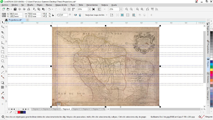
Figure 1. Position of the parallels of A_GI.

 

Table 3. Calculation of the scale of A_GI

No.	Parallels (°)		Position (mm)		Distance betweenthe parallels (mm)	Calculated scale	Estimated scale
1	6	5	71.81	59.48	12.33	9.011.354	9.000.000
2	2	1	23.48	11.37	12.1	9.178.093	9.200.000
3	-6	-5	-72.58	-60.69	11.89	9.340.899	9.300.000
4	-11	-10	-132.99	-121.12	11.87	9.359.784	9.400.000
5	-16	-15	-193.78	-181.81	11.97	9.278.496	9.300.000

 

Table 4. Calculation of the scale of B_SF

No.	Parallels (°)		Position (mm)		Distance between the parallels (mm)	Calculated scale	Estimated scale
1	11	10	99.78	90.75	9.03	12.299.092	12.300.000
2	6	5	55.21	46.11	9.09	12.216.602	12.200.000
3	2	1	18.55	9.21	9.33	11.897.419	11.900.000
4	-6	-5	-55.33	-46.33	9.00	12.344.183	12.300.000
5	-11	-10	-101.81	-92.24	9.56	11.611.453	11.600.000

 

Table 5. Calculation of the scale of C_LC

N°	Parallels (°)		Position (mm)		Distance between the parallels (mm)	Calculated scale	Estimated scale
1	6	5	54.32	45.33	8.98	12.363.413	12.400.000
2	2	1	18.15	9.03	9.12	12.179.107	12.200.000
3	-2	-1	-18.09	-8.94	9.14	12.152.466	12.200.000
4	-5	-4	-44.83	-35.96	8.87	12.523.669	12.500.000

 

Table 6. Calculation of the scale of D_EB

N°	Parallels (°)		Position (mm)		Distance between the parallels (mm)	Calculated scale	Estimated scale
1	2	1	21.4	10.34	11.06	10.045.203	10.000.000
2	-5	-4	-54.88	-43.7	11.18	9.935.616	9.900.000
3	-9	-8	-97.97	-86.59	11.38	9.757.618	9.800.000
4	-13	-12	-140.38	-129.66	10.71	10.368.607	10.400.000
5	-21	-20	-226.06	-215.18	10.88	10.211.377	10.200.000

Table 7. Calculation of the scale of E_KB

No.	Parallels (°)		Position (mm)		Distance between the parallels (mm)	Calculated scale	Estimated scale
1	13	12	216.31	199.81	16.5	6.733.939	6.700.000
2	9	8	149.96	133.32	16.64	6.675.678	6.700.000
3	5	4	83.62	66.85	16.76	6.626.312	6.600.000
4	-5	-4	-83.25	-66.64	16.61	6.688.538	6.700.000
5	-9	-8	-149.87	-133.26	16.6	6.690.552	6.700.000
6	-13	-12	-215.95	-199.35	16.6	6.691.358	6.700.000

 

With the estimated data, an average scale can be determined for each map and its corresponding standard deviation, which indicates the margin of error of the process (Table 8). This method is based on the dimensions described in table 2, if the values change depending on the source, the calculation must be carried out again.

 

Table 8. Mean scale and standard deviation

Map	Mean scale	Standard deviation
A_GI	9.240.000	+/- 150.000
B_SF	12.000.000	+/- 300.000
C_LC	12.300.000	+/- 150.000
D_EB	10.000.000	+/- 240.000
E_KB	6.700.000	+/- 50.000

 

3.2 Calculation of the meridian of origin

In Global Mapper, images were georeferenced using the meridian and parallel intersections as control points in the drawn grid of each map. The georeferenced images were imported to QGIS Desktop, in which the longitude of 15 or 20 locations were determined in the coordinate system of each map, depending on the case; after from these same locations its current longitude was determined taking Greenwich as the meridian of origin. Finally, in a calculation table the equation 1 was applied with the collected data, thus calculating the meridian of origin in reference to each of the locations (Table 9 to 11).

 

λorig = λG - (360° - λa) (1)

 

λorig: Longitude of the meridian of origin in relation to Greenwich.

λG: Longitude of the point relative to Greenwich, obtained from a current map.

λa: Longitude of the measurement point on the map.

 

For a better visualization of the process, a screenshot of the georeferenced map A_GI and the distribution of the locations taken as a reference for the calculation of the meridian of origin is included (Figure 2).

 

 

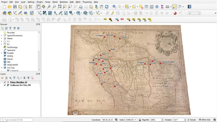
Figure 2. Distribution of the locations of A_GI.

 

 

Table 9. Calculation of prime meridian of A_GI

No.	Locations	λa (°)	360° - λa	λG (°)	λorig (°)
1	Bogotá	306.8	53.2	-74.07	-20.87
2	Borja	307.11	52.89	-77.55	-24.66
3	Caracas	311.88	48.12	-66.9	-18.78
4	Carthegene	304.04	55.96	-75.48	-19.52
5	Corupa	327.11	32.89	-51.62	-18.73
6	Cuenca	302.28	57.72	-80.00	-22.28
7	Curupatuba	324.62	35.38	-54.06	-18.68
8	Cuzco	309.37	50.63	-71.97	-21.34
9	Guayaquil	299.99	60.01	-79.89	-19.88
10	Jaen	304.24	55.76	-78.8	-23.04
11	Lima	302.75	57.25	-77.04	-19.79
12	Manta	298.55	61.45	-80.7	-19.25
13	Maracaibo	309.04	50.96	-71.61	-20.65
14	Napo	303.27	56.73	-77.81	-21.08
15	Pará	328.42	31.58	-48.49	-16.91
16	Pasto	302.25	57.75	-77.28	-19.53
17	Quito	301.38	58.62	-78.47	-19.85
18	S. Loüis de Maragnan	332.15	27.85	-44.26	-16.41
19	Trujillo	300.34	59.66	-79.03	-19.37
20	Zamora	303.55	56.45	-78.95	-22.5

 Table 10. Calculation of prime meridian of B_SF

No.	Locations	λa (°)	360° - λa	λG (°)	λorig (°)
1	Bogotá	300.61	59.39	-74.07	-14.68
2	Borja	297.3	62.7	-77.55	-14.85
3	Cuenca	294.00	66.00	-80.00	-14.00
4	Curupa	325.07	34.93	-51.62	-16.69
5	Curupatuba	322.5	37.5	-54.06	-16.56
6	Cuzco	300.39	59.61	-71.97	-12.36
7	Guayaquil	292.71	67.29	-79.89	-12.6
8	Jaen	294.44	65.56	-78.8	-13.24
9	Laguna	299.19	60.81	-75.67	-14.86
10	Lima	294.37	65.63	-77.04	-11.41
11	Napo	296.63	63.37	-77.81	-14.44
12	Negro	315.15	44.85	-60.01	-15.16
13	Pará	328.51	31.49	-48.49	-17.00
14	Pasto	294.73	65.27	-77.28	-12.01
15	Piura	291.57	68.43	-80.65	-12.22
16	Quito	293.39	66.61	-78.47	-11.86
17	Topayós	321.35	38.65	-54.94	-16.29
18	Truxillo	292.48	67.52	-79.03	-11.51
19	Xingú	324.74	35.26	-52.25	-16.99
20	Zamora	293.76	66.24	-78.95	-12.7

 

It should be added that the name of the locations was taken from each map, so there may be spelling mistakes or not coincidence with which it currently has. With the calculated data, an average λorig can be determined for each map and its corresponding standard deviation, which indicates the margin of error of the process (Table 12). In relation to the C_LC and D_EB maps, it was not necessary to carry out the previous procedure since each author described the meridian of origin used in their work.

 

Table 11. Calculation of prime meridian of E_KB

No.	Locations	λa (°)	λG (°)	λorig (°)
1	Bogotá	-76.45	-74.07	2.38
2	Borja	-78.64	-77.55	1.09
3	Cuenca	-81.93	-80.00	1.93
4	Cuzco	-74.28	-71.97	2.31
5	Guayaquil	-82.89	-79.89	3.00
6	Gurupa	-53.83	-51.62	2.21
7	Gurupatuba	-55.71	-54.06	1.65
8	Laguna	-76.36	-75.67	0.69
9	Lima	-79.21	-77.04	2.17
10	Napo	-79.29	-77.81	1.48
11	Pará	-50.64	-48.49	2.15
12	Quito	-81.2	-78.47	2.73
13	Truxillo	-81.78	-79.03	2.75
14	Xingú	-54.42	-52.25	2.17
15	Zamora	-81.61	-78.95	2.66

 

Table 12. Meridian of origin of the maps

Map	Mean λorig (°)	Standard deviation	Meridian of origin
A_GI	-20.16	+/- 1.98	Ferro (18° W)
B_SF	-14.07	+/- 1.94	Tenerife (16° W)
C_LC	—	—	Paris Observatory (2° E)
D_EB	—	—	London (0°)
E_KB	2.09	+/- 0.64	Paris Observatory (2° E)

3.3 Determination of the map projection

Using CorelDRAW, the grid drawn on each map was delineated for a better visualization of its shape and the angles formed between meridians and parallels. Then, the distances between each of the meridians and parallels were calculated, taking the left and upper sides of the map as a reference (Table 13 to 15). The origin of the measurements for the parallels is the equatorial line, for which positive positions are calculated for northern latitudes and negative positions for southern latitudes; in the case of meridians, the origin of the measurements is a random meridian from which the positions to its left are negative and to its right are positive. For a better visualization of the process, a screenshot of how A_GI map grid looks like is included (Figure 3).

 

 

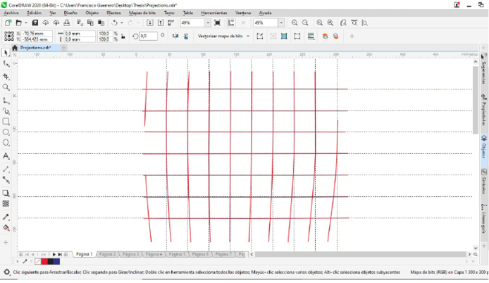
Figure 3. Drawn grid of A_GI.

 

Table 13. Distance between each meridian and parallel of A_GI

Parallels (°)	Position (mm)	Distance with the previous parallel (mm)		Meridian (°)	Position (mm)	Distance with the previous meridian (mm)
10	64.44	32.37		305	-96.36	32.1
5	32.06	32.06		310	-64.25	32.13
0	0	0		315	-32.11	32.11
-5	-32.31	32.31		320	0	0
-10	-64.67	32.36		325	31.75	31.75
-15	-97.35	32.67		330	63.95	32.2
-20	129.38	32.02		335	96.04	32.09
				340	127.62	31.58
				345	160.69	33.06

 

Table 14. Distance between each meridian and parallel of B_SF

Parallels (°)	Position (mm)	Distance with the previous parallel (mm)		Meridian (°)	Position (mm)	Distance with the previous meridian (mm)
10	93.06	45.76		200	0	0
5	47.3	47.3		205	47.29	47.29
0	0	0		300	94.06	46.77
-5	-47.46	47.46		305	141.43	47.37
-10	-94.6	47.14		310	187.94	46.51
				315	235.22	47.27
				320	282.19	46.96
				325	329.58	47.39
				330	376.54	46.96

 

Table 15. Distance between each meridian and parallel of D_EB

Parallels (°)	Position (mm)	Distance with the previous parallel (mm)		Meridian (°)	Position (mm)	Distance with the previous meridian (mm)
4	34.5	34.5		82	0	0
0	0	0		78	34.69	34.69
-4	-35.88	35.88		74	69.33	34.64
-8	-71.1	35.21		70	103.35	34.01
-12	-106.21	35.11		66	137.59	34.24
-16	-140.74	34.53		62	171.68	34.08
-20	-175.71	34.97		58	205.82	34.1
-24	-210.61	34.9		54	240.7	34.87
				50	275.14	34.44

 

With the drawn grid, the type of line with which the meridians and parallels were represented and the distance between each of them, the most probable map projection used was determined (Table 16). In relation to the C_LC and E_KB maps, it was not possible to carry out the previous procedure since each author did not depict any grid in their work.

  

Table 16. Projection of the maps

Map	Analysis of parallels	Analysis of meridians	Map Projection
A_GI	Straight lines that keep a uniform distance between each of them	Concave curves toward the central meridian, which appears to be located near the 320°. They keep a uniform distance between each of them	Sinusoidal
B_SF	Straight lines that keep a uniform distance between each of them	Straight lines that keep a uniform distance between each of them	Plate Carrée
D_EB	Equator is a straight line; other parallels are concave curves toward their respective pole and keep a uniform distance between each of them	Concave curves towards the central meridian, which appears to be located at 66°. They keep a uniform distance between each of them	Stereographic in equatorial aspect

3.4 Process of georeferencing and digitalization of the main features

The data determined in the previous process allowed to perform a correct georeferencing of the images using Global Mapper (Table 17). An adjustment was made with 4 control points for each of the maps, with the exception of the B_SF in which 6 control points were used. Once each one of the georeferencing process was finished and its correct execution was verified, the images were exported to GeoTIFF (.tif) format together with their corresponding PRJ file (.prj).

With the georeferenced images, the digitalization of the main features such as cities, rivers and coastlines began using the QGIS Desktop.12 Later, the Project Coordinate Reference System (CRS) was defined based on the parameters described in Table 17 and a GeoPackage (.gpkg) file was created to store the digitalized shapefiles.

The necessary shapefiles were created to represent the cities, rivers, and coastlines, setting the geometry type (point, line, or polygon) and the fields of the attribute table (name and level). Then, the digitization process was carried out, in the case of the cities and rivers, these elements were classified according to the symbology represented by each author in the original map, establishing categories in reference to their importance and flow, respectively. Finally, the attribute table was loaded with the map information and a particular style was defined for each shapefile that allows a quick identification of the entity it represents (Figure 4). Once the digitalization process was finished, the shapefiles were exported to GeoJSON (.geojson) format.

 

Table 17. Data to perform the georeferencing

Map	Map Projection	Meridian of origin	Central meridian
A_GI	Sinusoidal	Ferro (-18°)	316°
B_SF	Plate Carrée	Tenerife (-16°)	—
C_LC	Plate Carrée13	Paris Observatory (2°)	—
D_EB	Stereographic in equatorial aspect	London (0°)	-660
E_KB	Plate Carrée14	Paris Observatory (2°)	—

 

 

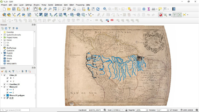
Figure 4. A_GI digitalized map.

 

3.5 Comparison of the maps

The process of comparing the maps was carried out using MapAnalyst, each image was imported and defining its resolution (dpi). Later, each one of the control points between the old map and OpenStreetMap15 was determined and a name was assigned that allows its identification. In relation to the control points, common locations were selected among the five maps in order to better visualize and interpret the results, these sites were easily identifiable cities and main river mouths that in few exceptions were not represented (Table 18).

 

Table 18. Locations of the control points

No.	Description	A_GI	B_SF	C_LC	D_EB	E_KB
1	city	Borgia	Borja	Borja	Borja	Borja
2	city	Cuenca	Cuenca	Cuenca	Cuenca	Cuenca
3	city	Guayaquil	Guayaquil	Guayaquil	Guayaquil	Guayaquil
4	city	Jaen	Jaen	Jaen	Jaen	Jaen
5	city	—	Laguna	Laguna	Laguna	Laguna
6	city	Lima	Lima	—	Lima	Lima
7	city	Loxa	Loxa	Loxa	Loxa	Loxa
8	river mouth	Madere	Madera	Madere	Madera	Madera
9	city	Manta	—	—	Manta	—
10	city	—	Napo	Napo	Napo	Napo
11	river mouth	—	Napo	Napo	Napo	Napo
12	river mouth	—	Negro	Negro	Negro	Negro
13	city	Para	Para	Para	Para	Para
14	river mouth	Parou	Parú	Parú	—	—
15	city	Payta	Payta	Payta	Payta	Payta
16	river mouth	Putomayo	Putomayo	Putomayo	Putomayo	Putomayo
17	city	Quito	Quito	Quito	Quito	Quito
18	river mouth	Tapaysos	Topayós	Topayós	Topayós	Topayós
19	river mouth	—	Tefe	Tefe	Tefe	Tefe
20	river mouth	Tocantins	Tocantin	Tocantin	Paranayba	Tocantin
21	city	Truxillo	Truxillo	—	Truxillo	Truxillo
22	river mouth	Yay	—	Yari	—	Yari
23	river mouth	Yurupau	Yurupa	Yurupa	Yurupau	—
24	city	Zamora	Zamora	Zamora	Zamora	Zamora

 

Once the control points were correctly determined and distributed, the compute option was selected, generating the graphical visualization of the comparison. The selected method was Displacements showing the variation of the position using Vectors & Circles at a scale factor of 1 (Figure 5). When each one of the comparison processes was finished, the images were exported to JPEG (.jpg) format.

 

 

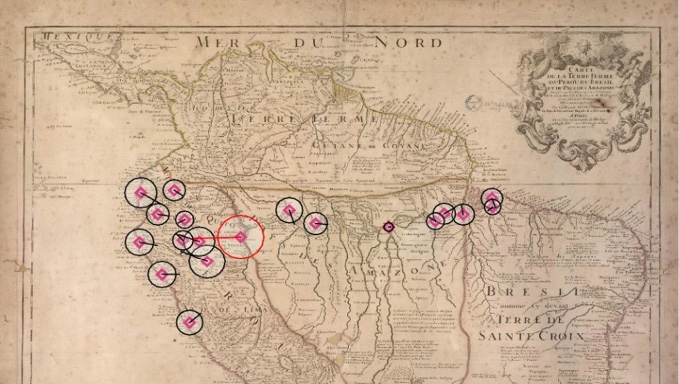
Figure 5. Process of comparison of A_GI using MapAnalyst.

 

4. Presentation and discussion of the results

The discussion of the results is based on the maps prepared with the digitalized shapefiles viewed through ArcGIS Online and the images produced by the comparison made with MapAnalyst. A description and visual analysis of the main characteristics of the maps under study is presented.

4.1 A_GI map

Visibly there was a greater knowledge of the cities in Ecuador and Peru, while in the Amazon and the Brazilian coast there is a reduced number of these. The coastal profile on the Brazilian coast is not detailed, the islands at the river mouth do not match with reality and were represented by several fragmented islands.

Regarding the positional displacements, it can be observed that they exist to a greater extent in the area of Ecuador and Peru, being the location of S. Francois de Borgia (Borja) an outlier of the control points. This great difference that can be observed in the terms of positional displacement is because the author took different sources of consultation to carry out his work (in the map title the author described the names of the sources) (Figure 6).

 

 

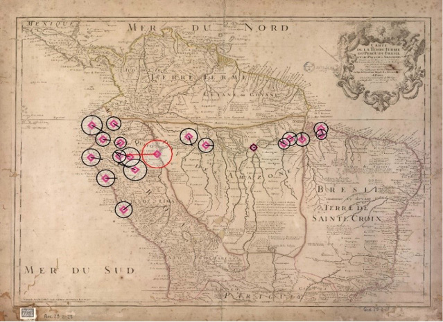
Figure 6. A_GI compared map. Source: National Library of Brazil.

 

 

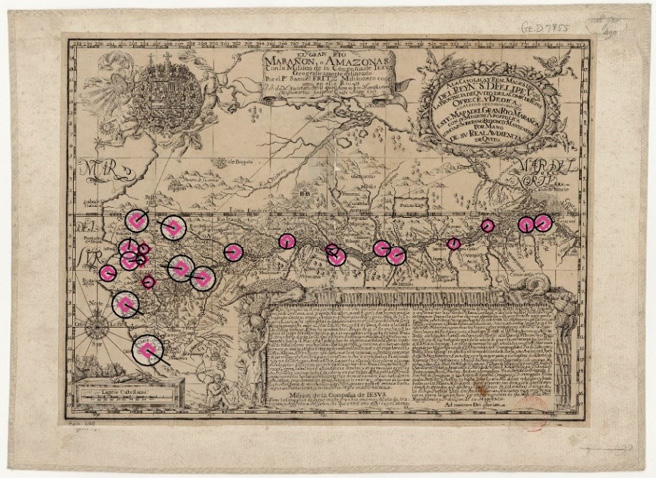
Figure 7. B_SF compared map. Source: National Library of France.

 

4.2 B_SF map

The map can be divided into two for an analysis starting from the central meridian to the west, in the Spanish territory an important level of detail is displayed, the opposite case occurs from the central meridian to the east (Portuguese territory). A greater knowledge of the cities in Ecuador and Peru is maintained, besides the first towns appear in the Amazon. The coastal profile has little accuracy with reality, the river mouth on the Brazilian coast was represented by countless islands of small and medium size.

The positional displacement shows the lower precision of the control points in Ecuador and Peru (presumably a bad longitudinal positioning), although clearly along the river course it can be presumed that there were adjustments in the determination of the position, that allowed greater precision between the Rio Negro and Paru river until reaching the mouth of the Amazon River (Figure 7).

4.3 C_LC map

Being the work of Samuel Fritz earlier, and in order to establish a comparison between it and his map, the author included the Amazon River course and its most important tributaries drawn by Fritz as a background (dotted line). More cities in the Amazon are included. The coastal profile does not match in the part of the Gulf of Guayaquil, being deformed towards the continent, the Isle des Joanes ou de Marayo (Ilha de Marajó) is represented at the river mouth in the Mer du Nord (Atlantic Ocean) surrounded by few small islands.

The positional displacement is variable, in Ecuador and the northern Peru a greater displacement is visualized except for Jaen and Borja compare with the locations near the Brazilian coast, the mouth of the Napo River is the outlier. It can be presumed that in several positions the measurements did not follow the same methodology, or they were not carried out and external data sources were taken as reference (Figure 8).

 

 

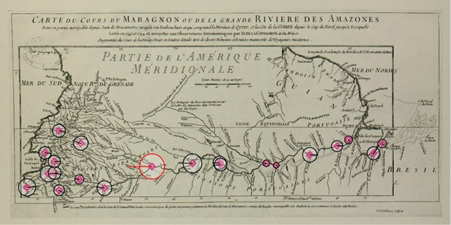
Figure 8. C_LC compared map. Source: National Library of France.

 

4.4 D_EB map

The map is part of a world atlas prepared by the author. According to his description the sources of consultation were French maps from which he took the information. More cities are included in the eastern part of Ecuador and Peru. In the Amazon and the Brazilian coast, main cities are consolidated, and secondary cities appear. The coastal profile in Ecuador and Peru is irregular, the river mouth in the Atlantic Ocean does not match with reality since it was represented by islands of medium and small extension with a latitudinal displacement of the entire area towards the south.

The positional displacement is variable, on the Ecuadorian and Peruvian coasts it is greater compared to the central zone of both countries, the city of Napo (Tena) and St. Francois d’ Borja (Borja) show the largest displacement while at the Topayos River mouth is the shortest. Finally, on the Brazilian coast a lower positional accuracy is visualized (Figure 9).

 

 

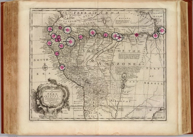
Figure 9. D_EB compared map. Source: National Library of Brazil.

 

4.5 E_KB map

A greater presence of cities is displayed on the Brazilian coast. The coastal profile in Ecuador and Peru is irregular considering that the river mouths towards the sea are wider and penetrate the continent. The Ins. De Joannes alias de Marayo (Ilha de Marajó) surrounded by few small islands was represented at the river mouth in the Mar Septentrio (Atlantic Ocean).

The author belonged to the same religious mission as Samuel Fritz, so it can be assumed that he had access to its reports and maps, therefore it is observed that basic information remains on the map supplemented with the data obtained from his explorations. The positional displacement is greater in Ecuador and Peru compare with the control points along the river course and the Brazilian coast, the Napus (Napo) River mouth is an outlier of the control points. From the Tefe River mouth to the Brazilian coast, the positional precision improves so adjustments may have been made in the determination of the position (Figure 10).

 

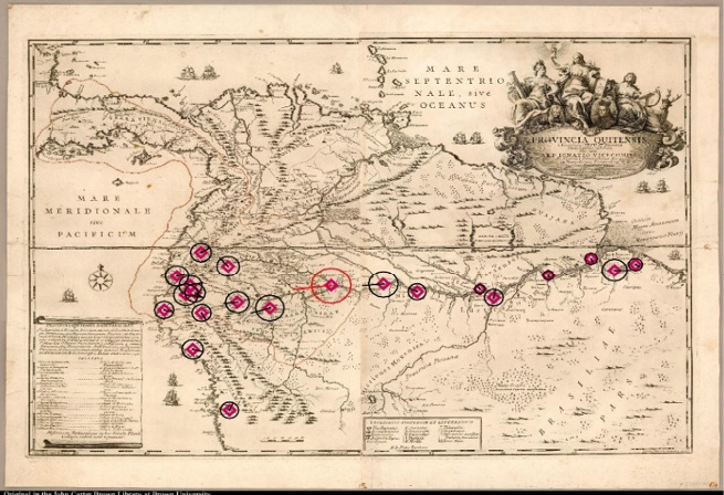
Figure 10. E_KB compared map. Source: National Library of France.

 

5. Visualization of the work

In order to visualize the information generated through a virtual environment, ArcGIS Online was used. The shapefiles in GeoJSON format were loaded one by one (cities, coastlines, and rivers) with the same style previously defined in QGIS Desktop, to have a reference to the current state of the terrain a base map of satellite images16 was defined. Once the five web maps had been created, it was chosen to make a web mapping application called Story Map Journal,17 in which the cartography generated and the most outstanding information of each author are shown at the same time. A brief summary is presented about the life of each author, a link to a website with their biography, a description and the bibliographic reference of the map made, and the map compared to the reality carried out in MapAnalyst.

 

6. Conclusions

The conclusions that can be formulated after the completion of this research are the following:

• QGIS Desktop is effective to rephrase an old map and have a digital version of its information stored for later use, preserving each of the characteristics such as prime meridian, central meridian, ellipsoid, projection, among others, with which the author prepared his work.
• The comparison of old maps is viable and can be done using specialized software, in this case MapAnalyst is a program that allows the user to carry out this task and through three different visualization methods (distortion grids, vectors of displacement, accuracy circles, and isolines) the correlation between an old map and reality can be established. This research focused on describing an analysis based on the geometric accuracy of old maps; however, there are other parameters that can be analyzed such as completeness, logical consistency, temporal quality, thematic accuracy, among others.
• The methodology to carry out this type of studies must be standardized in order to have specific parameters to be compared between the old map and the reality, which would allow an objective and precise analysis to be obtained for the formulation of the results.
• The visual and descriptive process for the comparison of old maps must necessarily be complemented with the inclusion of statistical tables and mathematical analyzes in relation to the position of the objects, with which the accuracy achieved, and its corresponding error will be calculated.

 

7. Bibliography

Barcelos, A. (2010). Jesuítas no Amazonas e no Orenoco: Explorações e polêmicas geográficas. Revista Eletrônica Documento Monumento, 3 (1), 74-88. https://www.ufmt.br/ndihr/revista/revistas-anteriores/revista-dm-03.pdf

Cintra, J. P. (2009). A cartografia digital como ferramenta para a cartografia histórica. Simpósio Luso-Brasileiro de Cartografia Histórica, 3.

Cintra, J. P., & Furtado, J. F. (2011). The Carte de l'Amerique meridionale of Bourguignon D'Anville: perspective axis of a compared Amazonian cartography. Revista Brasileira de História, 31(62), 273-316. https://doi.org/10.1590/S0102-01882011000200015

Dias, C. L. (2012). Jesuit maps and political discourse: The Amazon river of father Samuel Fritz. The Americas, 69 (1), 95-116. https://doi.org/10.1353/tam.2012.0052

Guillaume Delisle (2021) from Daniel Crouch Rare Books: https://www.crouchrarebooks.com/discover/mapmakers/delisle-guillaume

Harley, J. B. (1968). The Evaluation of Early Maps: Towards a Methodology. Imago Mundi, 22, 62–74. http://www.jstor.org/stable/1150436

Jenny, B. & Hurni, L. (2011). Studying cartographic heritage: Analysis and visualization of geometric distortions. Computers & Graphics, 35 (2), 402-411. https://doi.org/10.1016/j.cag.2011.01.005

Korányi, T. (2017). Brentán Károly Amazonas-térképe egy budapesti magángyűjteményben 2. https://blog.oszk.hu/foldabrosz/brentan-karoly-amazonas-terkepe-egy-budapesti-magangyujtemenyben-2

Lacza, T. (2000). Magyar jezsuiták Latin-Amerikában. Fórum Társadalomtudományi Szemle II.

Torres-Londoño, F. (2012). Visiones jesuíticas del Amazonas en la Colonia: de la misión como dominio espiritual a la exploración de las riquezas del río vistas como tesoro. Anuario Colombiano de Historia Social y de la Cultura, 39 (1), 183–213. https://revistas.unal.edu.co/index.php/achsc/article/view/34166

Vega Palma, A. (2010). Ríos y montes en la prefiguración del continente americano (1492-1548). http://repositorio.uchile.cl/handle/2250/123029